

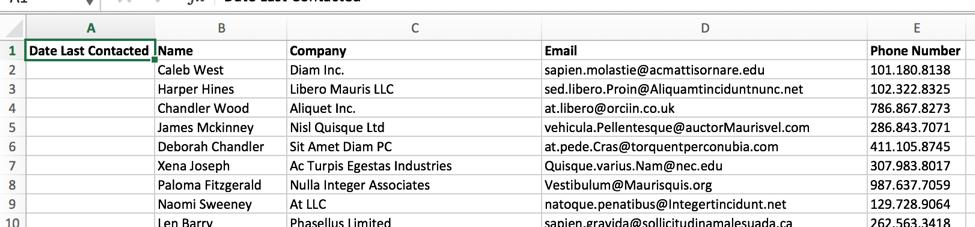
As a PR pro, Excel is probably your friend. But what happens if your media lists have information in one tab that you really need in another? Don’t go calling the intern just yet. This is where VLOOKUP comes into play.Let’s say in addition to your master list of targets, you also have separate lists to go along with each campaign or vertical. Or perhaps you divvy up your contacts and have tabs for each member of your team. Either way – it is easy to see how things can get messy. If there’s any overlap at all between lists, how can you be sure that any one reporter’s information is updated across all of your lists? Every reporter isn’t on every list, so sorting alphabetically won’t line the tables up for you to copy and paste. You could sort through the list by hand, but there are likely quite a few entries, so you’re looking at a pretty time-intensive task.Lucky for you, there is a quick way to get the information you need in one place: Excel’s VLOOKUP function.For this example, we have our master media list in one tab and our team’s outreach tracker in another. We want to combine the two data sets, showing both the reporter’s contact information and the date they were last contacted in the same sheet.1. Make sure both of your lists are in the same sheet to begin, on separate tabs:Note: All names and emails in the sample lists used are fictional.


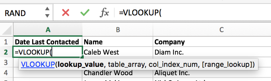
2. Insert a column into the first sheet where want to insert the information from the second. In this example, it’s the Date Last Contacted column:
3. In the first column, start entering your VLOOKUP formula:
A VLOOKUP is made up of four parts:Lookup_value: The value in this tab that you want to find in the second tab. The value that the two tabs share in this case will be the name of the reporter, which is found in B2.Table_array: Where will the lookup_value you just selected be found if it is within the second tab? Highlight the table in your second tab, making sure that the value you are looking up is the first column you select (left to right), and that you include all of the information you want to pull. When you select the table, you’ll see Excel automatically format the formula correctly with the names of your tab (so don’t worry too much about the quotes or exclamation points you see below).In our example, the tab is entitled “Last Contacted, and the information is found in A1:C201.

Since we always want the formula to look in this area (as opposed to moving dynamically when we apply the formula to other cells in our list), add a dollar sign in between the column and row designations. This will lock that value in and tell Excel to keep your table static.

col_index_num: Of the lookup table you just selected, which column contains the information you want displayed? Remember, the value the formula is looking for, in our case, their name, should have been selected as column 1.
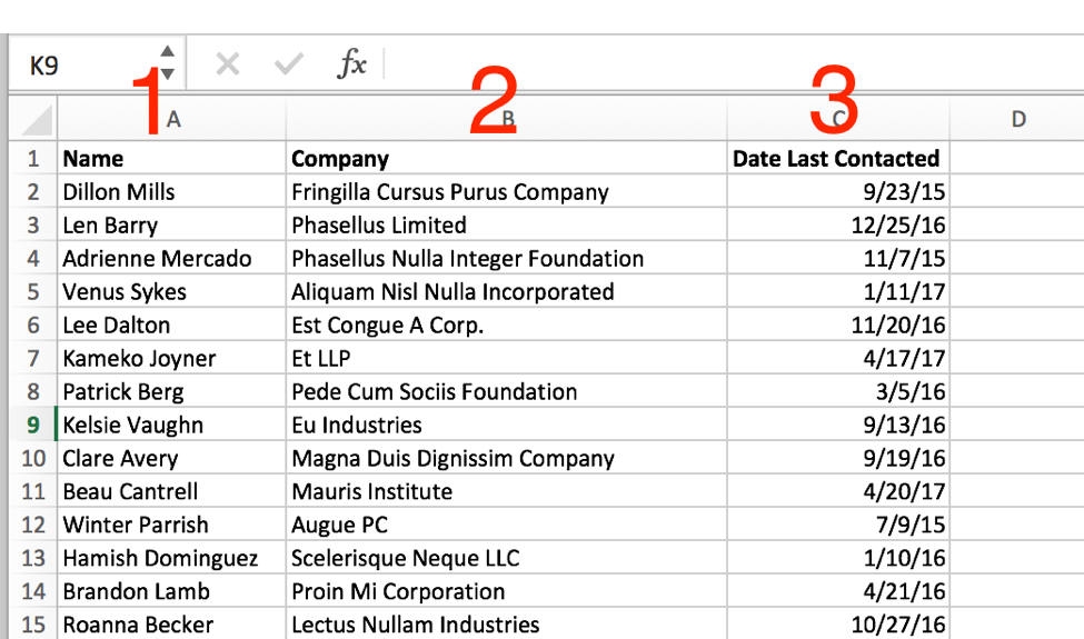
The information we want displayed once a match appears in column 1 will be found in column 3. Thus, our col_index_num will be 3.Range_Lookup: Do you want to make an exact match or a close match? The answer will either be TRUE or FALSE. TRUE will result in the data lookup being closely matched, FALSE will result in exact matches only. When you have data that has unique values (such as ID numbers or names), you will want to select FALSE.This last part is technically optional within of your formula, with the default being TRUE. If there is a chance that data within that column can be partially matched within itself, as is the case with names, you’re going to want to use FALSE.4. And with that, your formula is complete! Hit enter, and the information will populate. If Excel finds a match to your first row, you’ll see the new data appear in that cell.

Confirm it’s a match by searching in the other tab:

Now that the formula is confirmed to be working, double click the + in the bottom right corner of the cell to apply the formula to the rest of the table. This is where the $ step is important. If your column returns errors, or if you aren’t seeing the correct info, that is likely the culprit.
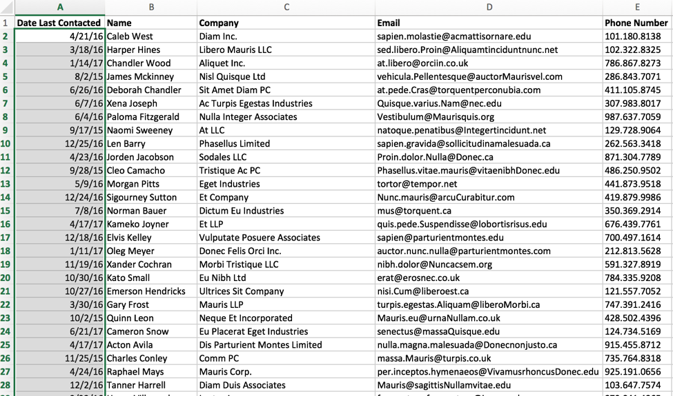
There you have it! Information from one tab “magically” inserted into the other. This is just one example of how to use the VLOOKUP function in Excel, but it has many practical applications! Have another use case for VLOOKUP in PR? Let us know in the comments!
What’s a Rich Text element?
The rich text element allows you to create and format headings, paragraphs, blockquotes, images, and video all in one place instead of having to add and format them individually. Just double-click and easily create content.
The rich text element allows you to create and format headings, paragraphs, blockquotes, images, and video all in one place instead of having to add and format them individually. Just double-click and easily create content.
Static and dynamic content editing
A rich text element can be used with static or dynamic content. For static content, just drop it into any page and begin editing. For dynamic content, add a rich text field to any collection and then connect a rich text element to that field in the settings panel. Voila!
How to customize formatting for each rich text
Headings, paragraphs, blockquotes, figures, images, and figure captions can all be styled after a class is added to the rich text element using the "When inside of" nested selector system.

